Query Store functionality in earlier versions of SQL Server

Aug 19, 2017 ~ dbafromthecold

One of the best features introduced in SQL Server 2016 was the Query Store. Having the ability to see which queries had regressed (gotten bad plans) over a period of time was pretty much a game changer imho. But many of us are still labouring away on earlier versions of SQL Server so we don’t get to work with this great new feature.

Until now, with the release of OpenQueryStore

If you haven’t heard of OpenQueryStore, it’s an open source project designed to, you guessed it, bring Query Store functionality to earlier versions of SQL Server (2008 to 2014).

When I heard about this project I immediately went onto the GitHub site, downloaded the repository and read through the installation instructions. I’ve been playing around with it for a while and this week was given a preview of the v2.0 release (which has now been released).

v2.0 provides two different install options for OpenQueryStore, Classic or Centralized.

Classic behaves in a similar fashion to Query Store in 2016 by monitoring an individual database whereas Centralized is installed in one “management” database and you specify which databases in the SQL instance you wish to monitor.

I went for Centralized mode and installation is a cinch, just download the repo and then run the Install.ps1 script: –

.\Install.ps1 -SqlInstance "SQL2012" -Database "DBA" -OQSMode "Centralized" -SchedulerType "SQL Agent"

After the script has run, the installer gives advice on what to do next: –

So I needed to INSERT a row into oqs.[monitored_databases] for each database I wanted to monitor, setup a schedule for the SQL Agent job (I set the job to run every minute), then run the UPDATE against oqs.[collection_metadata] and OpenQueyStore will begin collecting data.

A word of caution here. I used the SQL Agent data collection method. There is another option to run using Service Broker but if you do this the install script will run: –

ALTER DATABASE [<your db>] SET ENABLE_BROKER;

This requires an exclusive lock on the database so watch out!

After a while you’ll be able to run the reports that come with the download to get an overview of your system. This is the main dashboard: –

OpenQueryStore Main Dashboard

Here’s the Wait Stats report: –

OpenQueryStore Wait Statistics

These reports are great for a quick overview of the database monitored. Nicely laid out and with a quick glance I can see if there are any immediate causes for concern.

However, the real benefit of OpenQueryStore is in the data collected. The installation creates the following objects within the database: –

[oqs].[activity_log]
[oqs].[collection_metadata]
[oqs].[intervals]
[oqs].[monitored_databases]
[oqs].[plan_dbid]
[oqs].[plans]
[oqs].[queries]
[oqs].[query_runtime_stats]
[oqs].[wait_stats]

So there’s an absolute wealth of data to dig through! The reports provide query IDs so I can drop one into say: –

DECLARE @queryID SMALLINT;

SELECT TOP 1
    rs.[query_id]
    ,rs.[interval_id]
    ,rs.[last_execution_time]
    ,rs.[execution_count]
    ,rs.[avg_rows]
    ,rs.[last_logical_reads]
    ,rs.[avg_logical_reads]
    ,rs.[last_logical_writes]
    ,rs.[avg_logical_writes]
    ,q.[query_statement_text]
    ,p.[plan_handle]
FROM [oqs].[query_runtime_stats] rs
INNER JOIN [oqs].[Queries] q ON rs.[query_id] = q.[query_id]
INNER JOIN [oqs].[Plans] p ON q.[plan_id] = p.[plan_id]
WHERE rs.[query_id] = @queryID
ORDER BY rs.[interval_id] DESC;
GO

And then view all the execution stats of this query. Pretty cool, eh?

If you’re working with SQL Server versions 2008 to 2014 I’d highly recommend that you install this on a development box and start investigating the data that it’s collecting. As with any new system, set it up and monitor to see what it’s doing but I haven’t seen anything untoward.

The project is in (very) active development so keep an eye on the twitter account for more updates.

Thanks for reading!

Collation Conflicts

Jan 20, 2015 ~ dbafromthecold

I have recently seen some “bad plans” being generated by the optimiser and from investigation, the cause came down to the fact that the collation of the database where the queries were running was different to the tempdb collation.

Consider this situation, you have a stored procedure which collects various records and stores them in a temporary table. This temporary table is then used as a reference to delete records from another table in the database. This is a bit of a contrived example, but I just want to show you the impact differing collations can have.

N.B. – I’m running this in SQL Server 2012

First I’ll create a database with a different collation to the tempdb (the tempdb collation on my local instance is Latin1_General_CI_AS):-

CREATE DATABASE [CollationConflict] COLLATE SQL_Latin1_General_CP1_CI_AS;

Then I’ll create two tables in the database, populate them with data and create some nonclustered indexes.

Here’s the first table in the database:-

USE [CollationConflict];
GO

SET NOCOUNT ON;

IF EXISTS(SELECT 1 FROM sys.objects WHERE name = 'TableA')
    DROP TABLE dbo.[TableA];
GO

IF NOT EXISTS(SELECT 1 FROM sys.objects WHERE name = 'TableA')
    CREATE TABLE dbo.[TableA]
    (RecordID INT IDENTITY(1,1) PRIMARY KEY,
	Name VARCHAR(10));
GO

DECLARE @Counter	INT = 0;
DECLARE @Value		CHAR(10) = 'TEST';

WHILE @Counter <= 50000
BEGIN
    SET @Value = 'TEST' + CONVERT(VARCHAR(4),@Counter)

    INSERT INTO dbo.[TableA]
    (Name)
    VALUES
    (@Value);

    SET @Counter = @Counter + 1;
END

CREATE NONCLUSTERED INDEX [IX_TableA_Name] ON dbo.[TableA](NAME);
GO

And here’s the second table:-

IF EXISTS(SELECT 1 FROM sys.objects WHERE name = 'TableB')
    DROP TABLE dbo.[TableB];
GO

IF NOT EXISTS(SELECT 1 FROM sys.objects WHERE name = 'TableB')
    CREATE TABLE dbo.[TableB]
    (RecordID INT IDENTITY(1,1) PRIMARY KEY,
	Name VARCHAR(10));
GO

DECLARE @Counter	INT = 0;
DECLARE @Value		CHAR(10) = 'TEST';

WHILE @Counter <= 50000
BEGIN
    SET @Value = 'TEST' + CONVERT(VARCHAR(4),@Counter)

    INSERT INTO dbo.[TableB]
    (Name)
    VALUES
    (@Value);

    SET @Counter = @Counter + 1;
END

CREATE NONCLUSTERED INDEX [IX_TableB_Name] ON dbo.[TableB](NAME);
GO

To show the difference in plan’s generated, I’ll now create two temporary tables. The first one will use the same collation as tempdb but the second will be created with a different collation explicitly set.

Here’s the first temporary table using tempdb’s collation:-

CREATE TABLE #TempTableA
    (RecordID	 INT IDENTITY(1,1) PRIMARY KEY,
	Name		 VARCHAR(10));

DECLARE @Counter	INT = 0;
DECLARE @Value		CHAR(10) = 'TEST';

WHILE @Counter <= 500
BEGIN
    SET @Value = 'TEST' + CONVERT(VARCHAR(4),@Counter)

    INSERT INTO #TempTableA
    (Name)
    VALUES
    (@Value);

    SET @Counter = @Counter + 1;
END

CREATE NONCLUSTERED INDEX [IX_TempTableA_Name] ON #TempTableA(NAME);
GO

Here’s the second temporary table using same collation as the user database:-

CREATE TABLE #TempTableB
    (RecordID	 INT IDENTITY(1,1) PRIMARY KEY,
	Name		 VARCHAR(10) COLLATE SQL_Latin1_General_CP1_CI_AS);

DECLARE @Counter	INT = 0;
DECLARE @Value		CHAR(10) = 'TEST';

WHILE @Counter < 500
BEGIN
    SET @Value = 'TEST' + CONVERT(VARCHAR(4),@Counter)

    INSERT INTO #TempTableB
    (Name)
    VALUES
    (@Value);

    SET @Counter = @Counter + 1;
END

CREATE NONCLUSTERED INDEX [IX_TempTableB_Name] ON #TempTableB(NAME);
GO

Now I’m going to run two separate SQL statements which will reference the temp tables. The statements will perform the exact same operation, deleting a set of records from the main tables based on the records in the temp tables.

The only difference is that the COLLATE option is specified in the first (otherwise an error will be generated):-

DELETE A
FROM dbo.[TableA] AS A
INNER JOIN #TempTableA AS B ON A.Name = B.Name COLLATE Latin1_General_CI_AS
WHERE B.RecordID < 20;
GO

DELETE A 
FROM dbo.[TableB] AS A
INNER JOIN #TempTableB AS B ON A.Name = B.Name
WHERE B.RecordID < 20;
GO

The DELETE statements will generate the following plans when executed:-

The first query is scanning the nonclustered index. The properties of the DELETE operator show why:-

SQL is performing an implicit conversion, even though the COLLATE option was specified in the join. This is causing the nonclustered index scan. The impact of this can be seen by comparing the properties of the scan vs the seek in the second plan:-

The scan is reading all the records in the table, simply because of the implicit conversion!

So, if your user databases have a different collation than your tempdb ensure that you specify the correct collation when creating your temporary tables. Or just make sure your databases have the same collation as your SQL instance!

Cardinality Estimation in SQL Server

Nov 4, 2014 ~ dbafromthecold

Each time you view a seek/scan operator in an execution plan, you may have noticed that there’s a value for the estimated number of rows and a value for the actual number of rows. Sometimes these values can be fairly similar and sometimes they can be very different.

The estimated number of rows (or cardinality estimate) is very important when SQL is generating a plan to use for your query. It can mean the difference of your query running in milliseconds or minutes.

Quoting from Books Online:-

The query optimizer in SQL Server is cost-based. This means that it selects query plans that have the lowest estimated processing cost to execute. The query optimizer determines the cost of executing a query plan based on two main factors:

• The total number of rows processed at each level of a query plan, referred to as the cardinality of the plan.
• The cost model of the algorithm dictated by the operators used in the query.

The first factor, cardinality, is used as an input parameter of the second factor, the cost model. Therefore, improved cardinality leads to better estimated costs and, in turn, faster execution plans.

So, having an accurate value for the cardinality will allow SQL to generate a more efficient query plan which in turn will improve the performance of the query when executed. But how does the optimizer calculate the cardinality? Knowing how this value is calculated will allow you to write/tune queries more effectively.

I’ve got a few examples that will show the different values calculated in different scenarios. First, create a demo database:-

USE [master];
GO

IF EXISTS(SELECT 1 FROM sys.databases WHERE name = 'EstimatedRowsDemo')
    DROP DATABASE [EstimatedRowsDemo];
GO

IF NOT EXISTS(SELECT 1 FROM sys.databases WHERE name = 'EstimatedRowsDemo')
    CREATE DATABASE [EstimatedRowsDemo];
GO

Then create a table and insert some data:-

USE [EstimatedRowsDemo];
GO

IF EXISTS(SELECT 1 FROM sys.objects WHERE name = 'DemoTable')
DROP TABLE dbo.DemoTable;

IF NOT EXISTS(SELECT 1 FROM sys.objects WHERE name = 'DemoTable')
    CREATE TABLE dbo.DemoTable
	   (ColA INT,
	    ColB SYSNAME);
GO

INSERT INTO dbo.DemoTable
(ColA, ColB)
VALUES
(100 , 'VALUE1')
GO 200

INSERT INTO dbo.DemoTable
(ColA, ColB)
VALUES
(200 , 'VALUE2')
GO 500

INSERT INTO dbo.DemoTable
(ColA, ColB)
VALUES
(300 , 'VALUE2')
GO 400

Then create an index on the table:-

CREATE NONCLUSTERED INDEX [IX_DemoTable_ColA] on dbo.[DemoTable](ColA);
GO

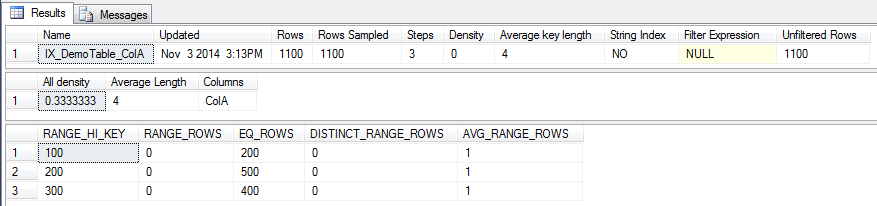
We can now look at the statistics on that index:-

DBCC SHOW_STATISTICS ('dbo.DemoTable','IX_DemoTable_ColA');
GO

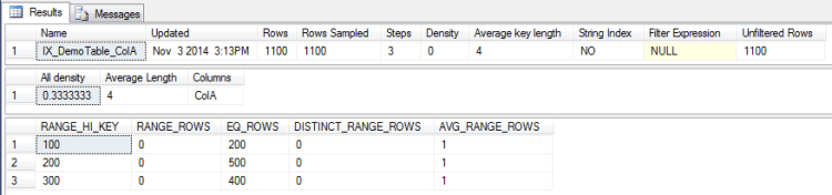
I’m not going to go through what each of the values means, the following article on Books Online explains each value:-
http://msdn.microsoft.com/en-us/library/hh510179.aspx

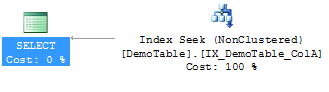
Now we can start running queries against the table and view the number of estimated rows value that the optimiser generates.

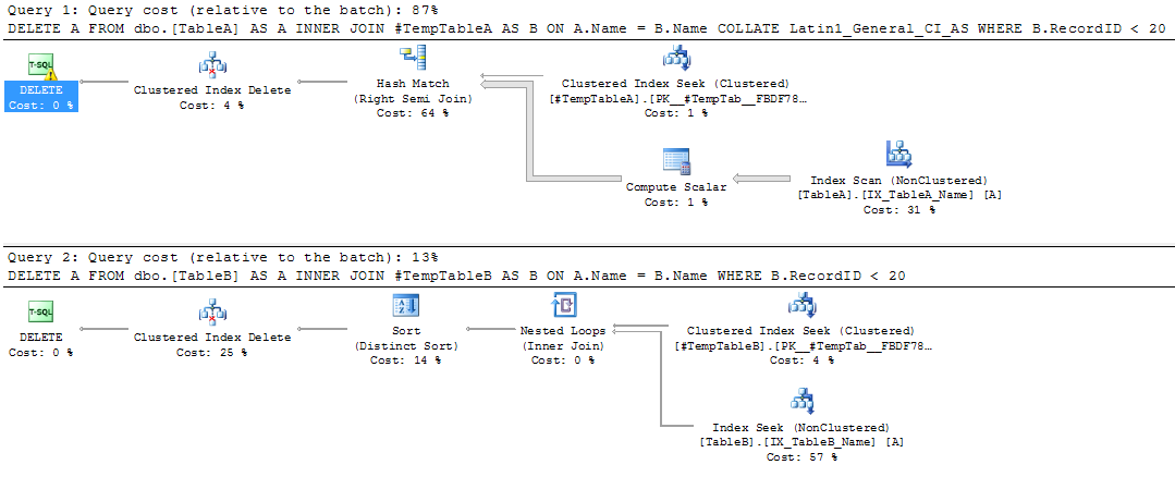
Quick note – All the queries are being run in SQL Server 2014 and will give the same execution plan:-

Remember, it’s the estimated number of rows generated for each one that we are interested in. Also, I’m running the following before each SELECT statement:-

DBCC FREEPROCCACHE;
DBCC DROPCLEANBUFFERS;

Don’t forget to click the ‘Include Actual Execution Plan’ button in SSMS (or hit Ctrl + M) as well.

OK, let’s go.

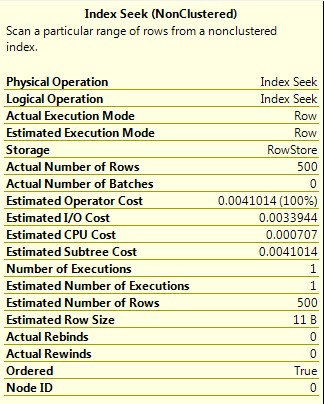
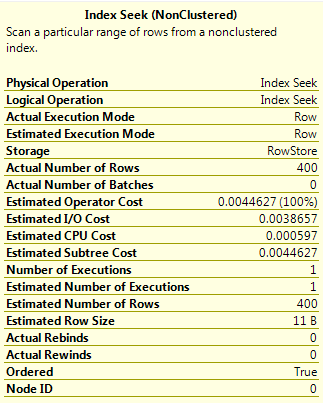
Query A

SELECT ColA FROM dbo.[DemoTable] WHERE ColA = 200;
GO

The value 200 corresponds to a RANGE_HI_KEY value in the stats for the index so the value for the EQ_ROWS is used, giving the estimated number of rows as 500.

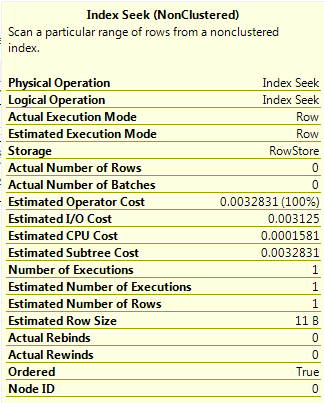
Query B

SELECT ColA FROM dbo.[DemoTable] WHERE ColA = 201;
GO

The value 201 is not one of the RANGE_HI_KEY values in the stats so the value for the AVG_RANGE_ROWS in the histogram step where the value would fall is used. This gives an estimated number of rows as 1, a significant difference from Query A.

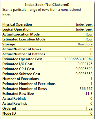
Query C

DECLARE @ParamA INT = 201;
SELECT ColA FROM dbo.[DemoTable] WHERE ColA = @ParamA;
GO

As a parameter is used in this query, the optimiser does not know the value set so the estimated number of rows is calculated as Density * Total Number of Rows (0.3333333 * 1100). This shows that using parameters in queries can drastically affect the estimated number of rows generated.

Query D

DECLARE @ParamA INT = 200;
SELECT ColA FROM dbo.[DemoTable] WHERE ColA > @ParamA;
GO

This query uses a parameter value but with an inequality operator (>). In this situation the estimated number of rows is 30% of the total number of rows in the table.

Query E

DECLARE @ParamA INT = 200;
SELECT ColA FROM dbo.[DemoTable] WHERE ColA > @ParamA OPTION(RECOMPILE);
GO

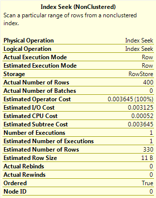
This is the same query as Query D but has OPTION(RECOMPILE) specified. This forces the plan to be compiled with the current value of the parameter, meaning that as the value is a RANGE_HI_KEY, the EQ_ROWS value for that histogram step is used. This gives a value of 400 for the estimated number of rows.

Query F

DECLARE @ParamA INT = 200;
DECLARE @ParamB INT = 300;
SELECT ColA FROM dbo.[DemoTable] WHERE ColA > @ParamA AND ColA < @ParamB
OPTION (QUERYTRACEON 9481);
GO

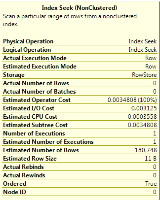
This query has two inequality operators. I specified OPTION (QUERYTRACEON 9481) to force SQL 2014 to use the old cardinality estimator, which will estimate the number of rows as 9% of the total number of rows in the able when two inequality operators are used.

When this query is run in SQL 2014 (using the new cardinality estimator) a different result for the estimated rows is generated. I’m unsure as to how this value is calculated, something that I will investigate in the future but for now it is just something to be aware of as the value is significantly different (180 vs 99).

EDIT

Kevan Riley (@KevRiley) contacted me about the new cardinality estimator for SQL 2014 and how it differs from the estimator in 2012.

For multiple predicates the estimator in 2012 used the formula:-

((Estimated number of rows for first predicate) *
(Estimated number of rows for second predicate)) /
Total number of rows

So for this query in 2012: (330 * 330)/1100 = 99

The new estimator in 2014 uses a formula with a process known as exponential backoff:

Selectivity of most selective predicate *
Square root of (selectivity of second most selective predicate) *
Total number of rows

So for this query in 2014: (330/1100) * (SQRT(330/1100)) * 1100 = ~180

Thank you very much Kevan

Query G

DECLARE @ParamA INT = 200;
DECLARE @ParamB INT = 300;
SELECT ColA FROM dbo.[DemoTable] WHERE ColA > @ParamA AND ColA < @ParamB OPTION(RECOMPILE);
GO

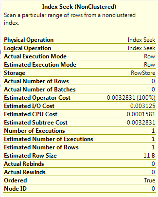
Finally, running the same query as Query F but using OPTION(RECOMPILE). This has the same effect as the result in Query E, the plan is compiled using the current values of the parameters. As there are two values, the optimiser takes a “slice” of the AVG_RANGE_ROWS values from the histogram steps that the parameter values fall across (1 in this simple example).

I hope these examples have shown you how the optimiser calculates the estimated number of rows in different scenarios. Please let me know if you have any feedback in the comments section.

Further information

This post is designed to give a brief introduction into cardinality estimation. There are literally hundreds on articles on the web about this subject, even more so now with the changes made in SQL 2014. Below are articles/posts I referenced to write this post.

Gail Shaw has a good presentation on this subject (which I referenced to write this post), it can be found here:-
http://www.sqlpass.org/24hours/2014/summitpreview/Sessions/SessionDetails.aspx?sid=7279

Paul White on multiple predicates for cardinality estimates:-
http://sqlperformance.com/2014/01/sql-plan/cardinality-estimation-for-multiple-predicates

Fabiano Amorim on getting the statistics used in a cached query plan:-
http://blogfabiano.com/2012/07/03/statistics-used-in-a-cached-query-plan/

DBA From The Cold

Ramblings on working as a SQL Server DBA

Category Archives: Query Tuning

Query Store functionality in earlier versions of SQL Server

Collation Conflicts

Cardinality Estimation in SQL Server